Finding Image Exposure Time - Advanced
This advanced work flow gives the most information and can provide more accurate results than the parity approach or the basic. It also sets you up for making better adjustment curves.
Advanced
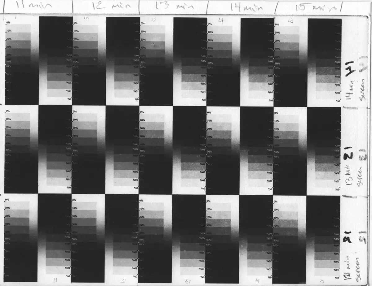
Find the Base Exposure Time needed to make a good aquatint matrix. Use that time to build an experiment in which both the exposure to the stochastic screen and the exposure to the image transparency is varied. This seems complicated, but it is just a more controlled version of the previous experiment.
The advanced version varies the intial Base Exposure Time (“screen” time), as well as the Image Exposure Time. It uses a transparency that has a series of step wedges. Those step wedges create a more nuanced exposure grid on the polymer plate (and resulting print).
First, the plate is exposed to the stochastic screen for three different potential screen times.
Second, the plate is exposed to the image (step wedges) for five different potential image times.
(screen) Base Exposure Times of: 12’, 13’, 14’
(image) Image Exposure times of: 11’ , 12’, 13’, 14’, 15
The notes I wrote on the back of the plate are:
Screen: 12’ 13’ 14’
Image: 11’ 12’, 13’, 14’, 15’
Fixxons transparency
Aristo Platinum Printer
Epson 3800
How the Advanced Option Works
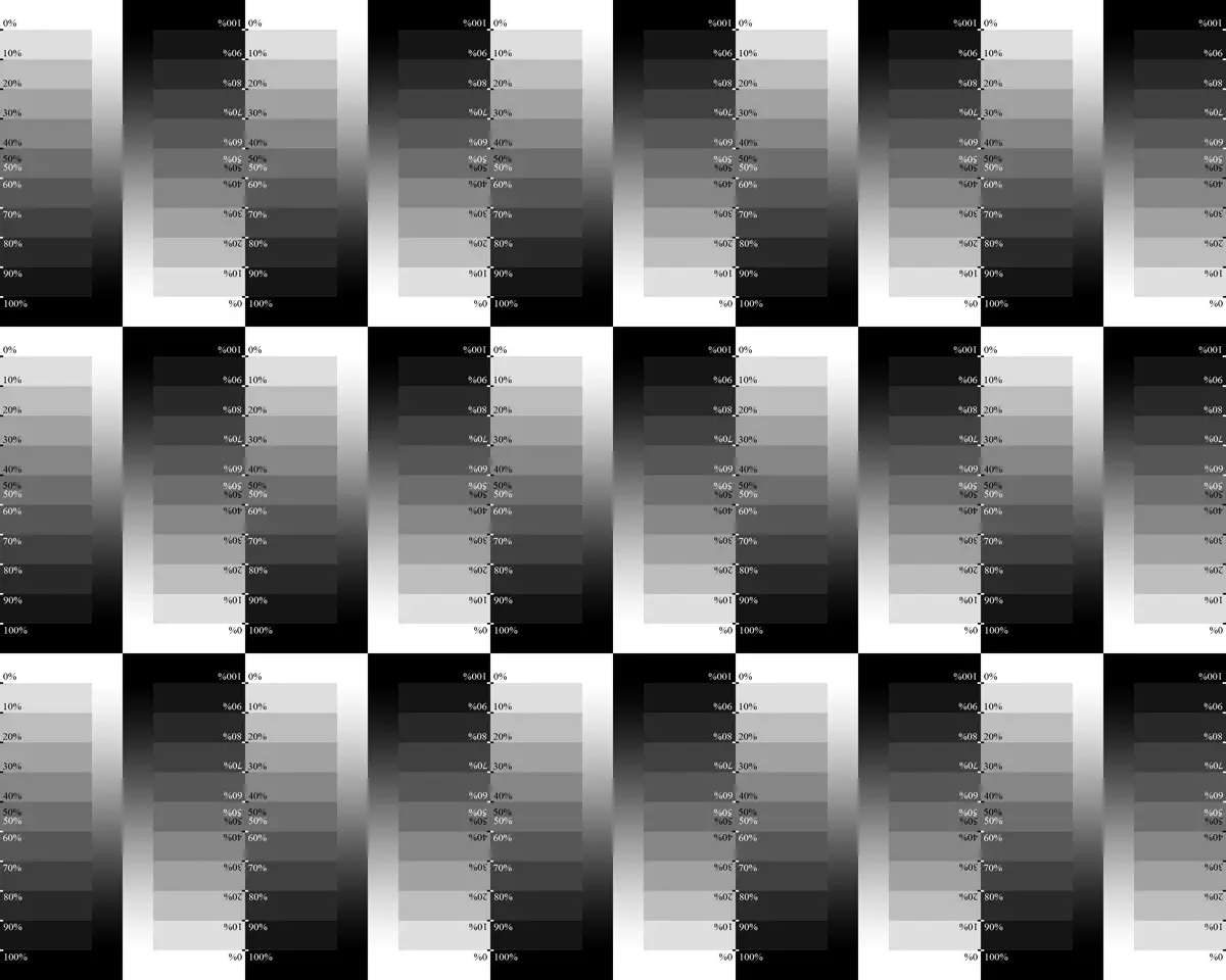
The advanced option uses the same principles as the previous option, with the addition of a variable Base Exposure time (“screen”). Here, you see a series of step wedges, lined up in a grid. The step wedges are paired in opposite directions. Each opposing pair will sit at the intersection of a specific Base Exposure Time (“screen”) and Image Exposure Time (“image”).
The following example shows “screen” times of 12, 13, 14 minutes and “image” times of 11, 12, 13, 14, 15 minutes using the Aristo Platinum Printer.
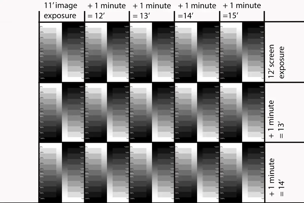
It’s set up for the resulting print to show 15 possible screen/image exposure times (in minutes).
screen/image
12’/11' 12’/12’ 12’/13’ 12’/14’ 12’/15’
13’/11’ 13’/12’ 13’/13’ 13’/14’ 13’/15’
14’/11’ 14’/12’ 14’/13’ 14’/14’ 14’/15’
A later experiment, not shown here, was run with a different exposure unit, in which this same image was exposed with “screen” times of 5, 6, 7 minutes and “image” times of 5, 6, 7, 8, 9 minutes. The results of this later experiment was used to make new adjustment curves using the technique demonstrated in the next section. The same process can be done with the results in this section.
Put the printed transparency on top of a polymer plate. Mark both the plate and the backing of the contact frame with screen and image times.
Replace the transparency with the stochastic screen. Leave 2 edges of the plate uncovered by the screen so you can see the exposure time notes that were made.
Make the initial exposure to the entire plate.
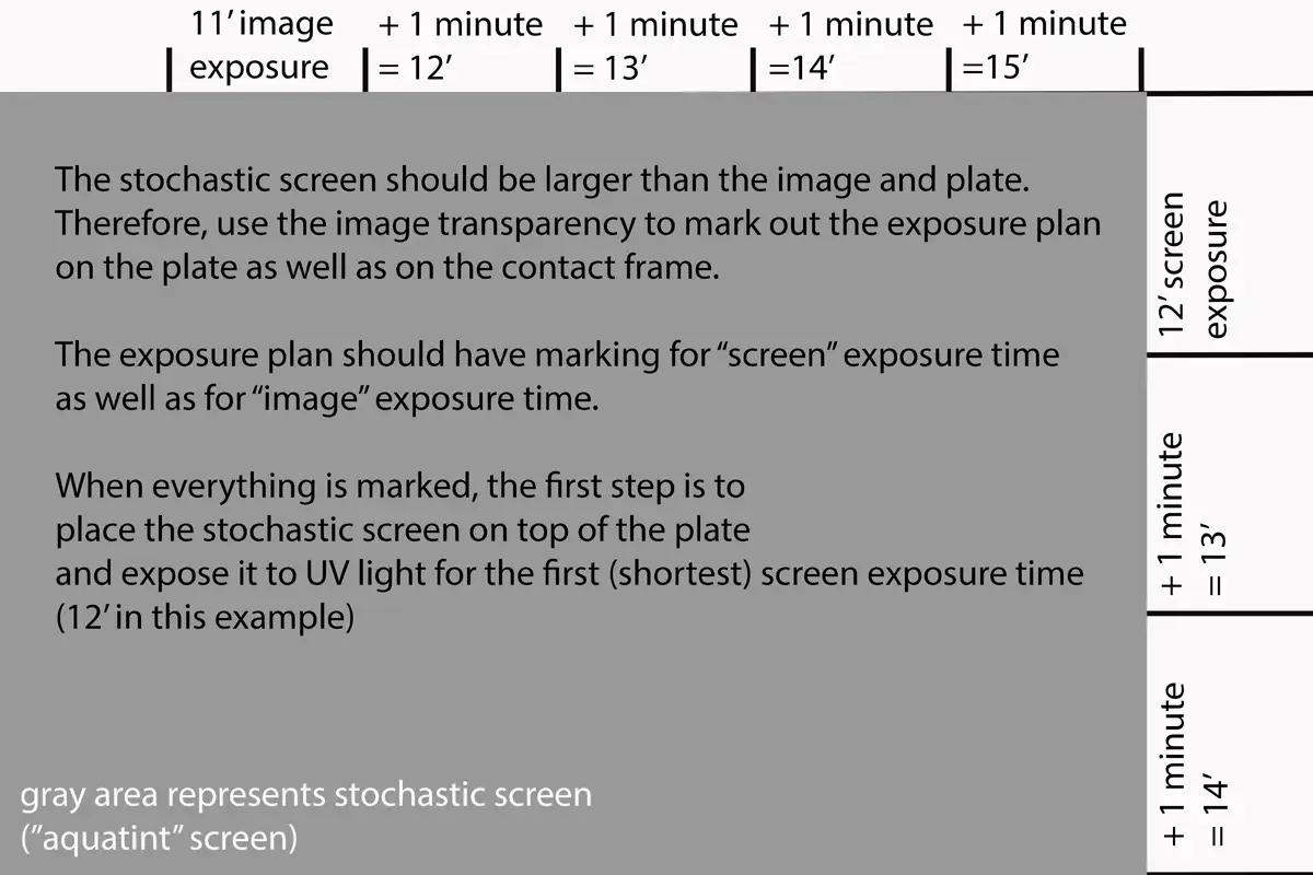
After the first exposure, cover part of the screen/plate with an opaque piece of plastic. Expose for 1 more minute.
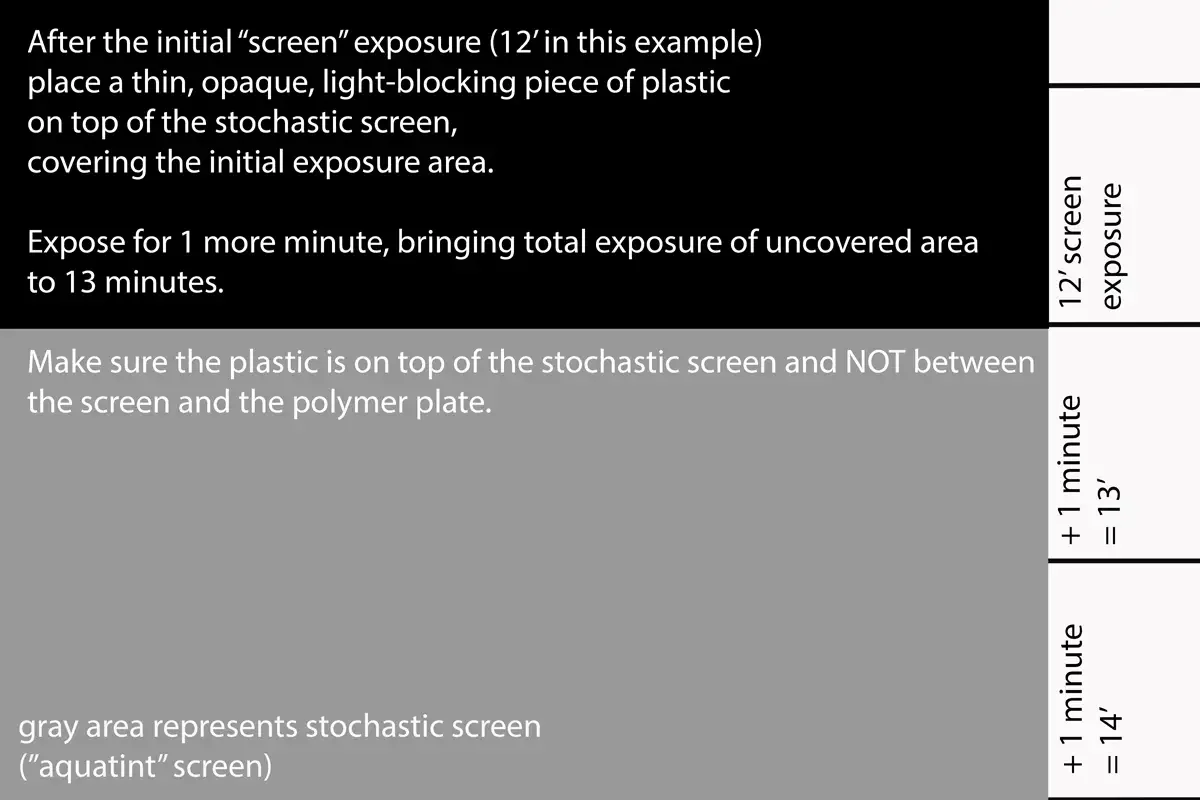
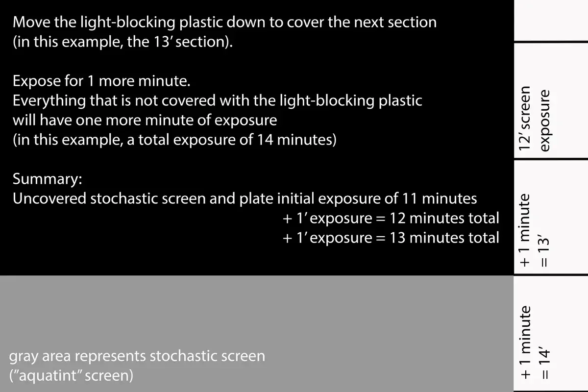
After exposure, move the plastic so it coveres the next zone and expose again for 1 minute.
After all screen exposures, replace the stochastic screen with the image transparency. Use the registration marks to line everything up. Make the initial exposure. (11’ minutes in this example)
Cover one strip with opaque plastic and expose for 1 more minute.
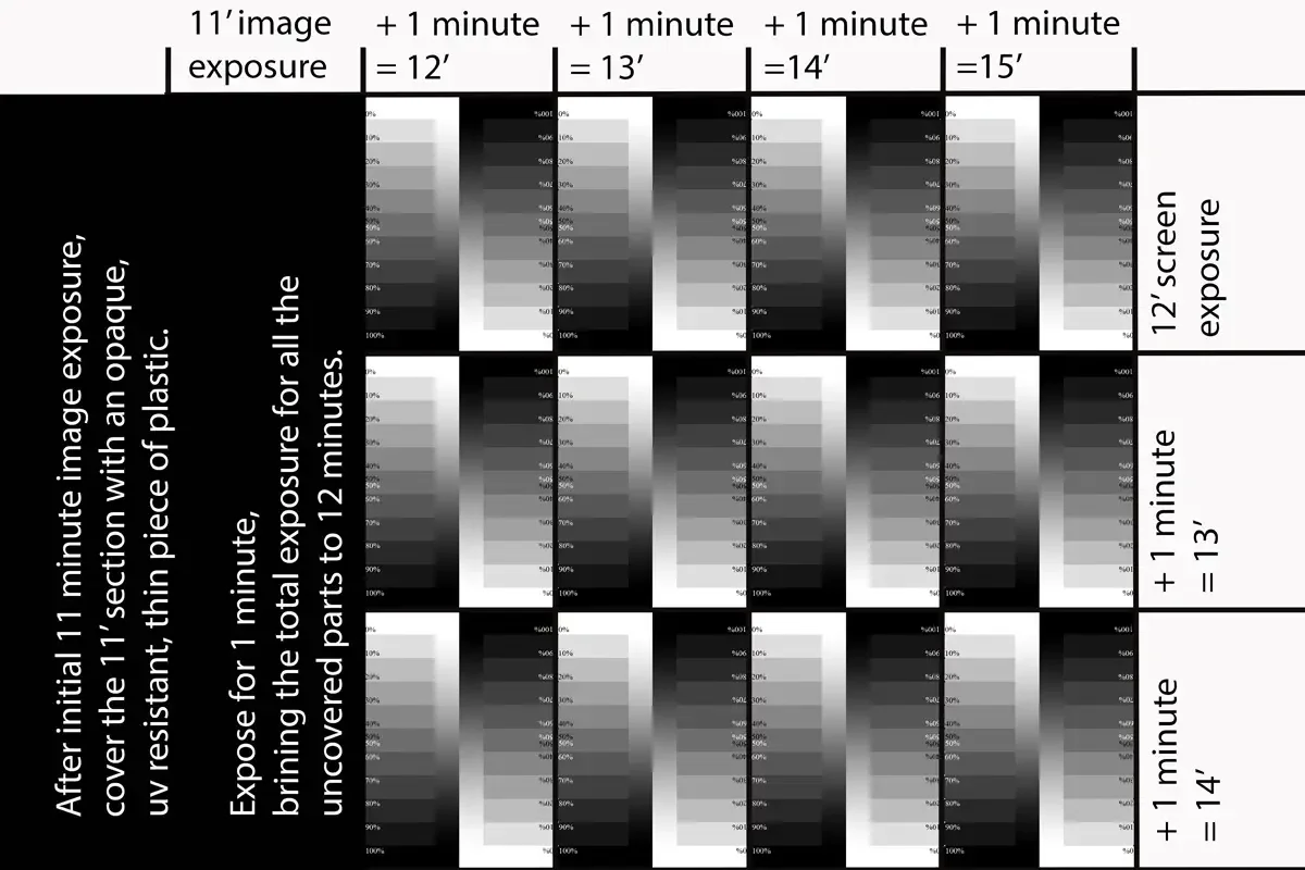
Move the opaque plastic to cover the next striip and expose again for 1 minute.
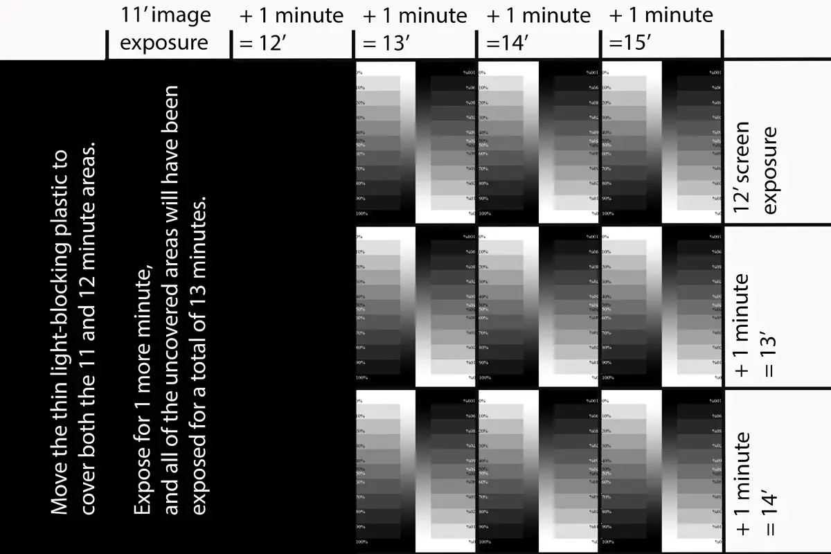
Move the opaque plastic to the next strip so it is covered (along with all the previous strips) and expose for 1 more minute.
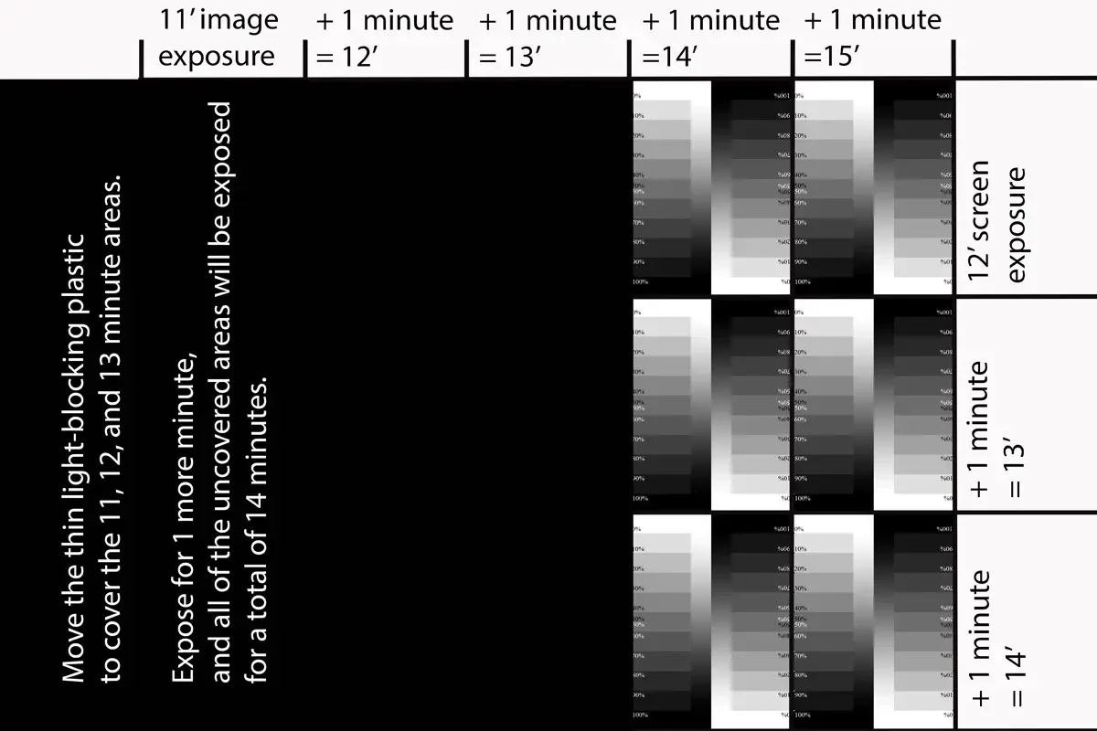
Repeat the process of moving the opaque plastic from strip to strip, making sure that, once covered, a strip stays covered. Keep track of all the additive exposures that are made so that times can be accurately tracked.
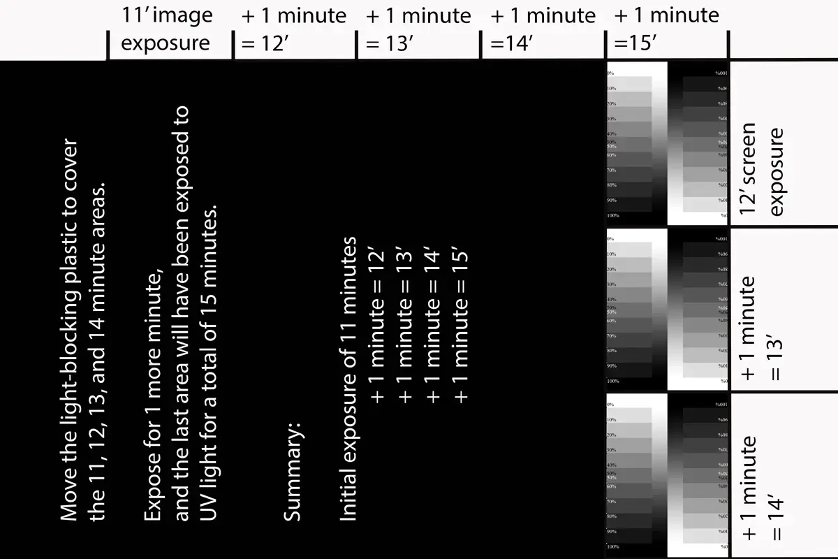
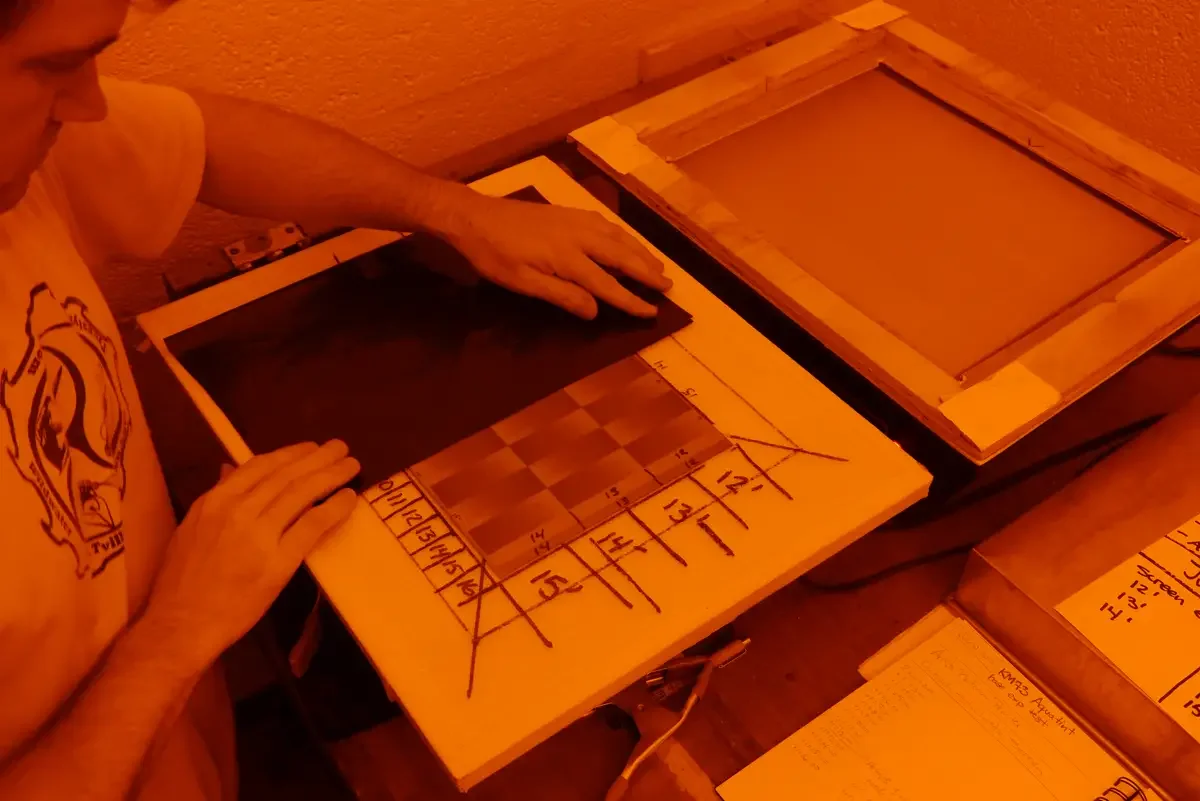
The previous images showed graphical represenations of this advanced option experiment. The next images will show real photos of the experiment being performed.
Screen exposure times are made in horizontal strips while image exposure times are along vertical strips.
Place the KM73 plate on the contact frame and remove the protective film.
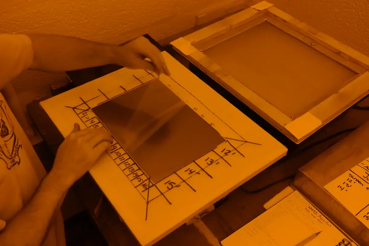
Place the stochastic screen on top of the plate. Printed side of the stochastic screen goes against the polymer side of the plate.
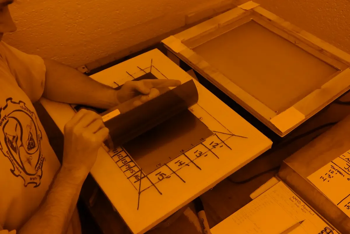
Make the initial “aquatint” exposure to the plate, using the shortest time planned for the stochastic screen.
In this example, the shortest “screen” time is 12 minutes, so that is the first exposure made, to the entire plate with the stochastic screen.
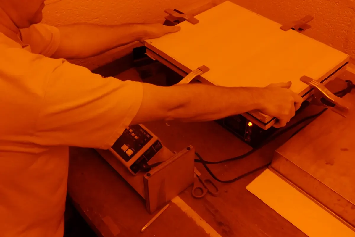
Cover the first horizontal strip after the first exposure and make another exposure of 1 minute.
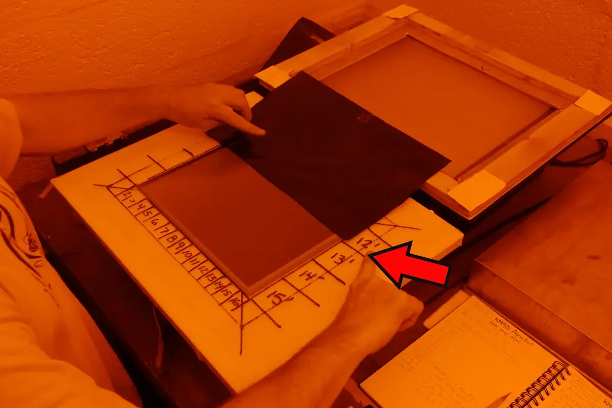
Cover the first and second horizontal strips with the opaque plastic and make another exposure of 1 minute.
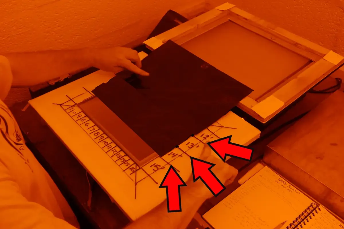
When all of the screen exposures have been made, remove the stochastic screen and replace it with the image transparency. Carefully line it up with the registration marks made earlier.
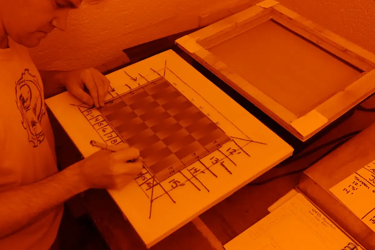
Make the initial exposure to the entire plate. The initial exposure is the lowest total desired exposure planned for the experiment.
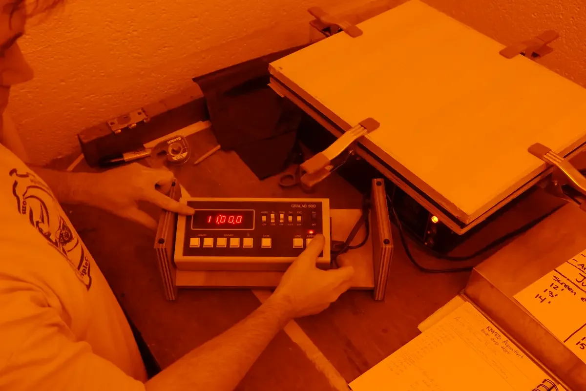
After the initial exposure, cover the first vertical strip, and make another exposure of 1 minute.
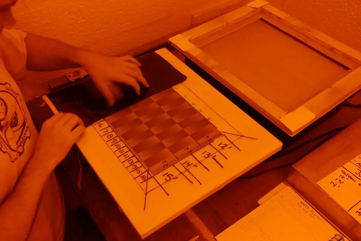
Cover the first and second vertical strips and expose for 1 minute.
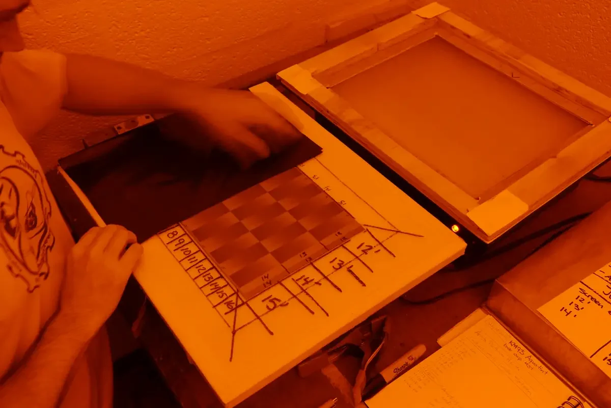
Cover the first, second, and third vertical strips and expose for 1 minute.
Repeat the process until all but one vertical strip is exposed for one more minute.
Cover the first, second, and third vertical strips and expose for 1 minute.
Repeat the process until all but one vertical strip is exposed for one more minute.
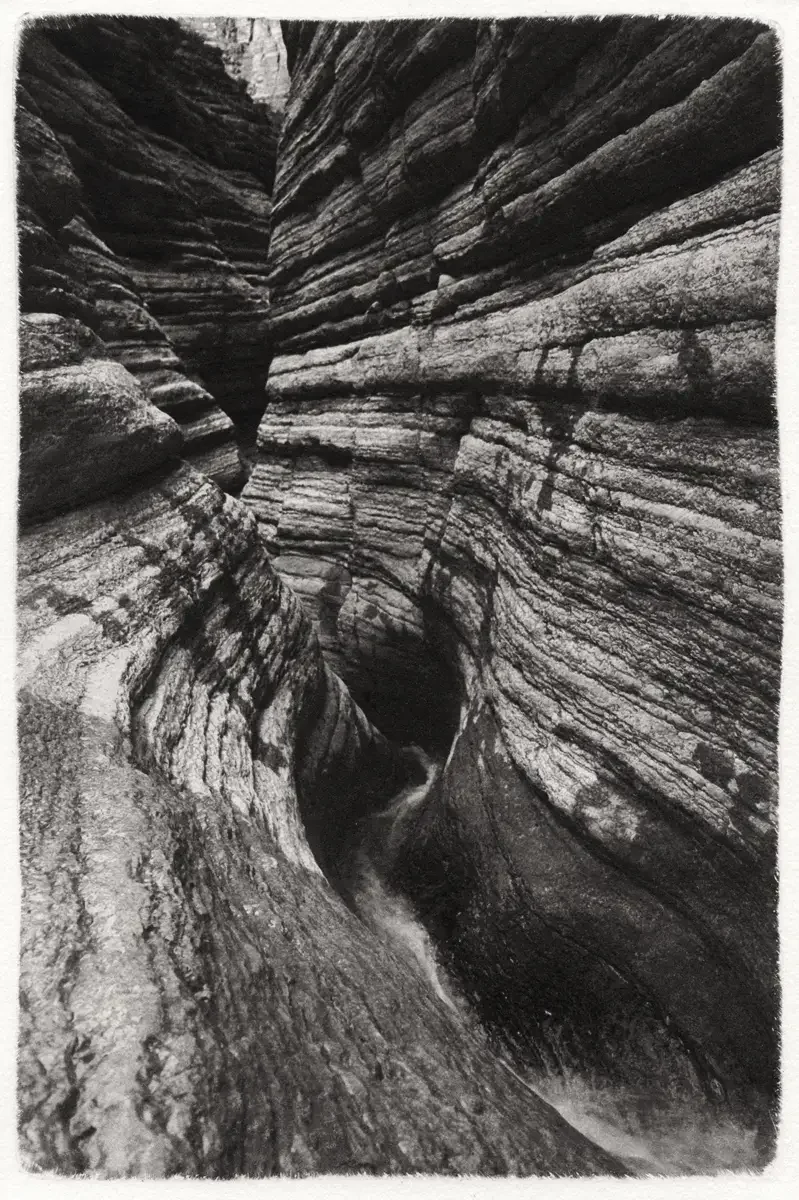
Let the print dry before examining it. Contrast changes slightly as the print dries. After it is dry, however, take a close look at the grid of step wedges. Choose the one that has the largest tonal range. Write down the screen and image times that work best, and use those to make some real photographs with this technique. Save this print (along with all other experiments) for future reference as you make and fine-tune adjusment curves.